Introduction Tucked away in the Arabian Gulf, Bahrain may be a small island nation, but its cultural richness speaks volumes. Bahrain has roots that run deep in history. Its traditions have gracefully evolved into modern life. Bahrain offers a unique blend of old and new. The warmth of its people is inviting. The rhythm of its music is captivating. The aroma of its cuisine tantalizes the senses. Bahrain’s culture is an experience waiting to be explored.
1. A Tapestry of Heritage Bahrain’s cultural identity is shaped by its strategic position as a trading hub. For centuries, it has welcomed influences from Persia, India, Africa, and Europe. This diverse heritage is evident in its architecture. Its language is a fusion of Arabic dialects, spiced with Persian, English, and Hindi.
The ancient Dilmun civilization once flourished here. The legacy lives on in archaeological sites like the Bahrain Fort (Qal’at al-Bahrain). This site is now a UNESCO World Heritage Site.
✈️ Planning your next adventure? Don’t let complicated bookings slow you down! I always use Expedia to find the best flight deals—fast, reliable, and super easy to compare prices. Whether you’re jetting off to a tropical paradise or hopping over to your next city escape, book your tickets hassle-free through Expedia and start your journey right
2. The Heartbeat of Hospitality Bahrainis are known for their generous hospitality. It’s not uncommon for strangers to be welcomed with Arabic coffee (qahwa) and dates. The traditional majlis is a sitting room for receiving guests. It remains a core element in Bahraini homes. It symbolizes respect, storytelling, and community.
3. Music, Dance & the Arts The traditional music of Bahrain is especially notable. Fidjeri (sailor songs) pay tribute to the island’s pearl diving past. Instruments like the oud (a string instrument) and tabla (drum) are commonly used, creating soulful rhythms that echo across generations.
Bahrain also fosters a vibrant contemporary arts scene. The country hosts the annual Spring of Culture festival. It also boasts a growing number of art galleries. Bahrain is a hub for regional creatives.
4. The Taste of Bahrain Bahraini cuisine is a reflection of its multicultural heritage. Dishes such as machboos (spiced rice with meat) and muhammar (sweet rice served with fried fish) are loved by many. Harees (a wheat and meat dish) is also a beloved staple. The use of spices like saffron, cardamom, and cinnamon brings a fragrant warmth to every bite.
And let’s not forget the street food. You can find everything from shawarma stalls to fresh juices. Traditional sweets like halwa are also available. There’s always something flavorful to try.
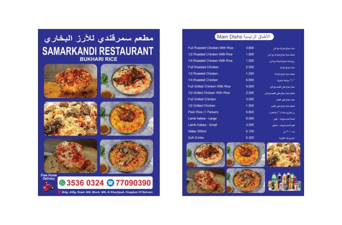
Experience Authentic Bukhari Rice at Our Restaurant in Sitra, Bahrain
If you’re in Sitra, Bahrain, and craving a delicious, aromatic, and flavorful meal, look no further than our restaurant! We specialize in serving Bukhari Rice, a traditional Middle Eastern dish that’s loved by locals and tourists alike. It’s the perfect comfort food. It combines fragrant basmati rice with tender, marinated meat. Everything is cooked to perfection with a mix of spices.
In this blog post, we’ll share a little bit about the rich history of Bukhari Rice. We will provide a few recipes and cooking tips. We’ll also showcase why our version is a must-try.
Bukhari Rice
What is Bukhari Rice?
Bukhari Rice is a flavorful rice dish often served with lamb, chicken, or beef. It’s a staple of many Middle Eastern cuisines, particularly in countries like Saudi Arabia, Kuwait, and Bahrain. The dish is traditionally prepared by cooking the rice with marinated meat. The meat is often seasoned with spices like cumin, cinnamon, and turmeric. The rich, aromatic flavors come together as the rice absorbs the meat’s juices during cooking.
At our restaurant, we take pride in our Bukhari Rice. We use fresh, high-quality ingredients. This creates a truly mouthwatering meal.
Watch Us Prepare Bukhari Rice
To give you a sneak peek of the magic behind our Bukhari Rice, check out these videos where you can see the process in action:
These videos showcase our signature method, which highlights the importance of fresh ingredients, careful preparation, and traditional cooking techniques. You might be curious about the spices we use. Alternatively, you may want to see how we assemble the dish. These clips give you a glimpse into our kitchen.
Bukhari Rice Recipe: How to Make It at Home
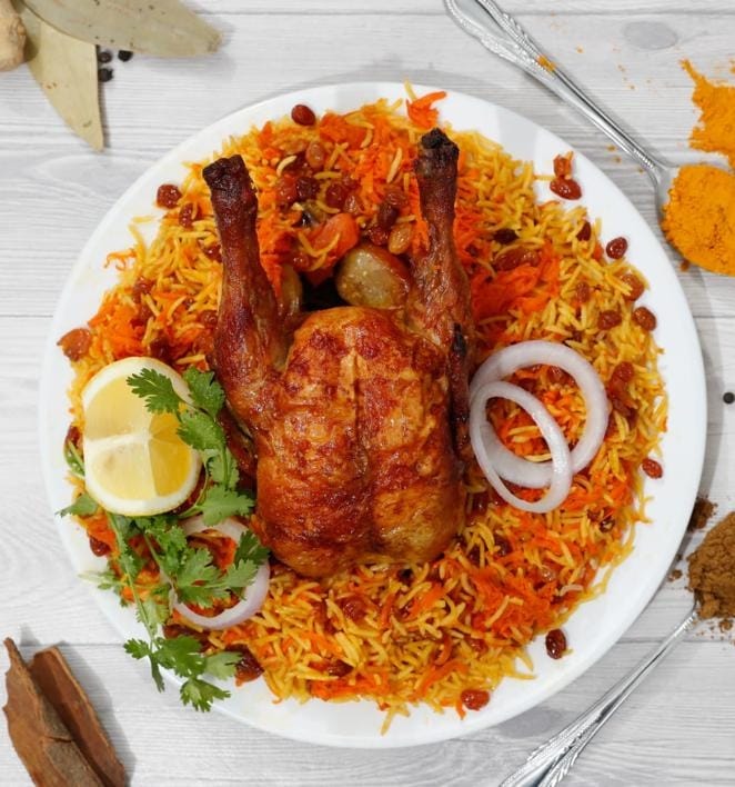
Chicken with bukhari rice
If you’d like to try making Bukhari Rice yourself, here’s a simple recipe to get you started.
Ingredients:
2 cups basmati rice
500g chicken (or lamb, beef, your choice)
1 large onion, finely chopped
2 tomatoes, chopped
3 cloves garlic, minced
1 tbsp cumin
1 tbsp cinnamon
1 tsp turmeric
3 tbsp vegetable oil
4 cups chicken stock (or water)
Salt and pepper to taste
A handful of raisins (optional, for sweetness)
A few slivers of almonds (for garnish)
Instructions:
Prepare the Rice: Wash the rice under cold water until the water runs clear. Soak it for about 20 minutes and set it aside.
Cook the Meat: In a large pot, heat the oil and sauté the onions and garlic until golden brown. Add the meat and cook it until browned on all sides. Add the chopped tomatoes, cumin, cinnamon, turmeric, salt, and pepper. Let the meat cook with the spices for about 10 minutes.
Simmer: Pour in the chicken stock (or water) and bring it to a boil. Lower the heat and cover the pot. Let the meat simmer until tender. It takes about 45 minutes for chicken and longer for lamb or beef.
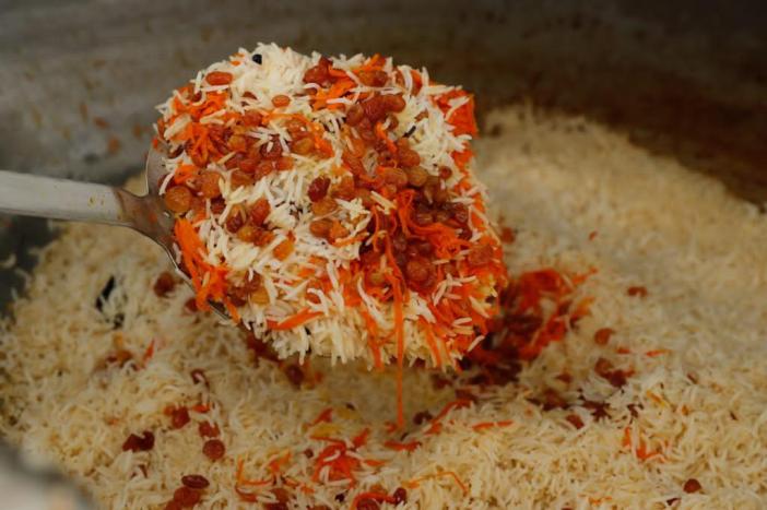
Cook the Rice: Add the soaked rice to the pot with the meat. Stir gently, ensuring the rice is evenly distributed. Cover and cook on low heat until the rice is fully cooked and has absorbed the flavors (about 20 minutes).
Final Touches: Optionally, toast the raisins and almonds in a small pan with a little oil. Scatter them over the rice before serving. This adds an extra touch of sweetness and texture.
“This isn’t just roasted chicken—it’s Sitra’s Sunday ritual. Samarkandi’s whole chicken emerges crackling-gold from the clay oven, skin glistening with cumin and cardamom. Served atop aromatic Bukhari rice studded with almonds, this is Bahraini comfort food that hugs you back.”
Serve the Bukhari Rice hot with a side of yogurt. You can also serve it with a fresh salad. Enjoy a meal that will take your taste buds on an unforgettable journey.
Samarkandi Bahrain Sitra
Tips for Cooking Perfect Bukhari Rice
Use Basmati Rice: For that signature fluffy texture and fragrant aroma, basmati rice is essential.
Soak the Rice: Always soak your rice for at least 20 minutes. This helps it cook more evenly. It also prevents it from becoming too sticky.
Perfectly Spiced: Don’t be afraid to adjust the spices to your preference. The key is balancing the cinnamon, cumin, and turmeric for that deep, warm flavor.
Don’t Skip the Meat Marinade: Marinate your chicken, lamb, or beef for a few hours with spices. This process will infuse it with maximum flavor. A simple marinade with garlic, cumin, and olive oil works wonders.
Simmer Slowly: The slow simmering of the meat is crucial. Let it absorb the flavors of the spices to create that rich, deep taste in your rice.
Optional Garnishes: For extra flavor and texture, garnish with fried almonds, raisins, or even crispy onions.
Why Our Bukhari Rice Stands Out
What makes our Bukhari Rice so special? We believe in delivering a meal that is rich in flavor. It is also crafted with love and attention to detail. Our chefs use only the best ingredients. We pride ourselves on providing an authentic experience. This experience transports you straight to the heart of the Middle East.
Whether you’re a local or visiting Bahrain, stop by our restaurant in Sitra. Try our signature Bukhari Rice. It’s a dish that promises to satisfy both your hunger and your craving for something deliciously different!
bahrain
5. Faith and Festivities Islam plays a central role in daily life. You’ll hear the call to prayer echoing across cities, and Friday remains a sacred day for family and prayer. However, Bahrain is also known for its religious tolerance. It hosts diverse communities, including Christians, Hindus, and Jews, who worship freely.
Cultural celebrations like Eid, Ramadan, and National Day are major events, often accompanied by fireworks, performances, and community gatherings.
6. Modern Bahrain: Embracing Change While proud of its traditions, Bahrain is also forward-thinking. Bahrain was the first Gulf nation to discover oil. It was the first to host a Grand Prix. The nation is also among the first to empower women in politics and business. Skyscrapers rise beside traditional souqs. Luxury malls sit close to heritage sites. This is a symbol of how Bahrain balances modernity with cultural preservation.
When I visited Petra, I found that booking a guided day trip to Amman made everything much easier. If you’re planning something similar, this link has some great tour options you can explore.
Conclusion Bahrain isn’t just a destination — it’s a cultural mosaic where the past and present coexist in harmony. Whether you’re strolling through the alleys of Muharraq, sipping tea by the corniche, or watching a traditional dance at a village wedding, you’ll find yourself touched by the soul of Bahrain — warm, resilient, and timeless.
Want this turned into a visual blog, Instagram carousel, or even a YouTube script? I can help with that too!
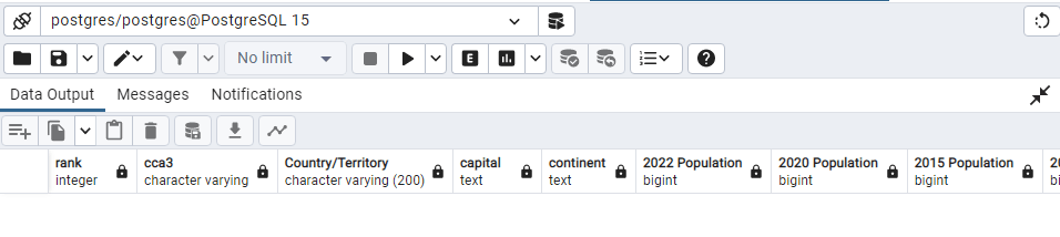
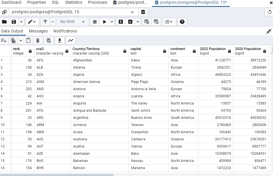
FROM ‘C:\Users\laxmi\Downloads\world_population.csv’
WITH (FORMAT CSV, HEADER);
SELECT * FROM public.world_population;
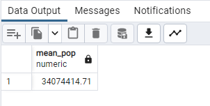
SELECT ROUND (AVG(“2022 Population”),2) AS mean_pop
FROM public.world_population;
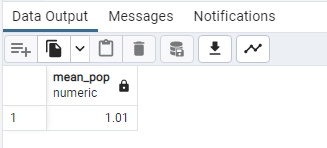
SELECT ROUND (AVG(“Growth Rate”),2) AS mean_pop
FROM public.world_population;
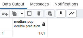
SELECT
PERCENTILE_CONT(0.5) WITHIN GROUP (ORDER BY “Growth Rate”) AS median_pop
FROM public.world_population;
SELECT
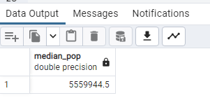
PERCENTILE_CONT(0.5) WITHIN GROUP (ORDER BY “2022 Population”) AS median_pop
FROM public.world_population;
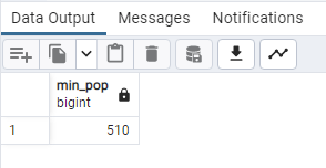
SELECT
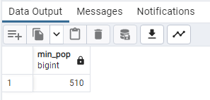
MIN(“2022 Population”) AS min_pop
FROM public.world_population;
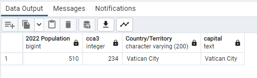
SELECT “2022 Population” ,”rank” “cca3”, “Country/Territory”, “capital” FROM world_population WHERE “2022 Population” = ‘510’;
–So Vatican City has minimum population–
SELECT
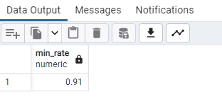
MIN(“Growth Rate”) AS min_rate
FROM public.world_population;
ALTER TABLE public.world_population ALTER COLUMN “Growth Rate” TYPE Numeric USING “Growth Rate”::Numeric;
OR
SELECT “Growth Rate”, CAST (“Growth Rate” AS Numeric( 10,2))
FROM public.world population
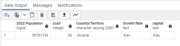
SELECT “2022 Population” ,”rank” “cca3”, “Country/Territory”, “capital” “Growth Rate” FROM world_population WHERE “Growth Rate” = ‘0.91’;
_–Minimum Growth rate is in Ukraine Kiev–
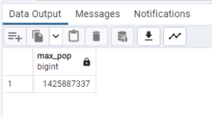
SELECT
MAX(“2022 Population”) AS Max_pop
FROM public.world_population;
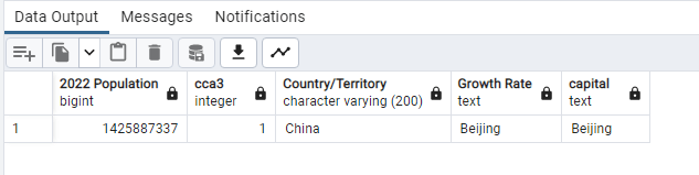
SELECT “2022 Population” ,”rank” “cca3”, “Country/Territory”, “capital” “Growth Rate”,”capital” FROM world_population WHERE “2022 Population” = ‘1425887337’;
–So miximum population in 2022 was China Beijing–
SELECT MIN(“2022 Population”) AS Min_pop FROM public.world_population;
SELECT
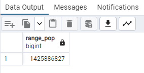
MAX(“2022 Population”) – MIN(“2022 Population”) AS range_pop
FROM public.world_population;
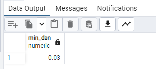
SELECT MIN(“Density (per km²)”) AS Min_den FROM public.world_population;
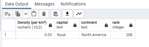
SELECT (“Density (per km²)”), “capital”, “continent”, “rank” FROM world_population WHERE (“Density (per km²)”) <= ‘0.03’
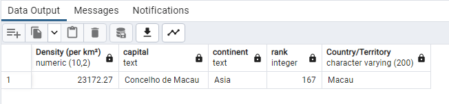
SELECT (“Density (per km²)”), “capital”, “continent”, “rank”, “Country/Territory” FROM world_population WHERE (“Density (per km²)”) >= ‘23172.27’;
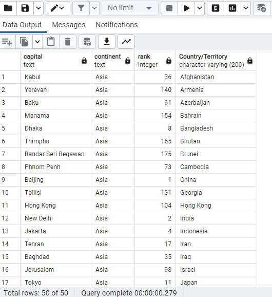
SELECT “capital”, “continent”, “rank”, “2022 Population” “Country/Territory” FROM world_population WHERE (“continent”) = ‘Asia’;
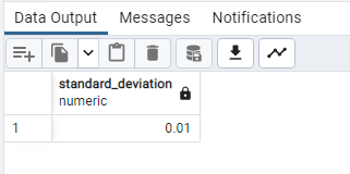
SELECT
ROUND(STDDEV(“2020 Population”), 2) AS standard_deviation
FROM public.world_population;
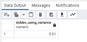
SELECT
ROUND(SQRT(VARIANCE(“Growth Rate”)), 2) AS stddev_using_variance FROM public.world_population;
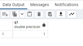
SELECT PERCENTILE_CONT(0.25) WITHIN GROUP (ORDER BY “Growth Rate”) AS q1 FROM public.world_population;
WITH mean_median_sd AS
(
SELECT
AVG(“2022 Population”) AS mean,
PERCENTILE_CONT(0.5) WITHIN GROUP (ORDER BY “2020 Population”) AS median,
STDDEV(“2022 Population”) AS stddev
FROM public.world_population
)
SELECT
ROUND(3 * (mean – median)::NUMERIC / stddev, 2) AS skewness
FROM mean_median_sd;
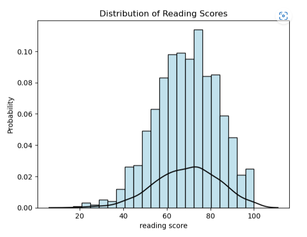
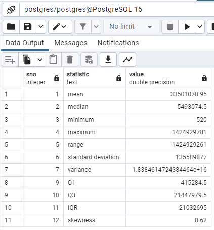
WITH RECURSIVE summary_stats AS ( SELECT ROUND(AVG(“2020 Population”), 2) AS mean, PERCENTILE_CONT(0.5) WITHIN GROUP (ORDER BY “2020 Population”) AS median, MIN(“2020 Population”) AS min, MAX(“2020 Population”) AS max, MAX(“2020 Population”) – MIN(“2020 Population”) AS range, ROUND(STDDEV(“2020 Population”), 2) AS standard_deviation, ROUND(VARIANCE(“2020 Population”), 2) AS variance, PERCENTILE_CONT(0.25) WITHIN GROUP (ORDER BY “2020 Population”) AS q1, PERCENTILE_CONT(0.75) WITHIN GROUP (ORDER BY “2020 Population”) AS q3 FROM public.world_population ), row_summary_stats AS ( SELECT 1 AS sno, ‘mean’ AS statistic, mean AS value FROM summary_stats UNION SELECT 2, ‘median’, median FROM summary_stats UNION SELECT 3, ‘minimum’, min FROM summary_stats UNION SELECT 4, ‘maximum’, max FROM summary_stats UNION SELECT 5, ‘range’, range FROM summary_stats UNION SELECT 6, ‘standard deviation’, standard_deviation FROM summary_stats UNION SELECT 7, ‘variance’, variance FROM summary_stats UNION SELECT 9, ‘Q1’, q1 FROM summary_stats UNION SELECT 10, ‘Q3’, q3 FROM summary_stats UNION SELECT 11, ‘IQR’, (q3 – q1) FROM summary_stats UNION SELECT 12, ‘skewness’, ROUND(3 * (mean – median)::NUMERIC / standard_deviation, 2) AS skewness FROM summary_stats ) SELECT * FROM row_summary_stats ORDER BY sno;
SELECT
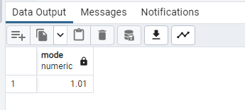
MODE() WITHIN GROUP (ORDER BY “Growth Rate”) AS mode
FROM public.world_population;
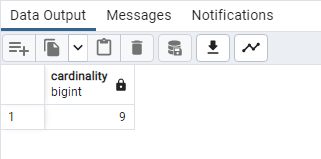
SELECT
COUNT(DISTINCT “Growth Rate”) AS cardinality
FROM public.world_population;
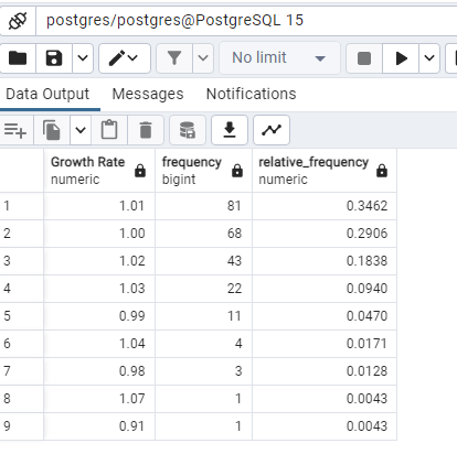
–Periodicity and relative periodicity Using GROUP BY and COUNT in Postgres, we can determine how often each category appears in a categorical field. In order to calculate the relative frequency, we will utilize a CTE to count all of the values in the rating column. We’ll utilize CTE because not all databases allow window functions. We’ll also go over how to use window functions to calculate relative frequency.–
WITH total_count AS
(
SELECT
COUNT(“Growth Rate”) AS total_cnt
FROM public.world_population
)
SELECT
“Growth Rate”,
COUNT(“Growth Rate”) AS frequency,
ROUND(COUNT(“Growth Rate”)::NUMERIC /
(SELECT total_cnt FROM total_count), 4) AS relative_frequency
FROM public.world_population
GROUP BY “Growth Rate”
ORDER BY frequency DESC;
–The count of values in the rating field is captured by a CTE in the example above. The percentage/relative frequency of each category in the rating field was then determined using it. We’ll explore a less complicated method of computing relative frequency utilizing window functions as Postgres supports them. The total number of values in the rating field is determined by adding the counts of ratings across each category, which we will do using the OVER() function.–
SELECT
“Growth Rate”,
COUNT(“Growth Rate”) AS frequency,
ROUND(COUNT(“Growth Rate”)::NUMERIC / SUM(COUNT(“Growth Rate”)) OVER(), 4) AS relative_frequency
FROM public.world_population
GROUP BY “Growth Rate”
ORDER BY frequency DESC;
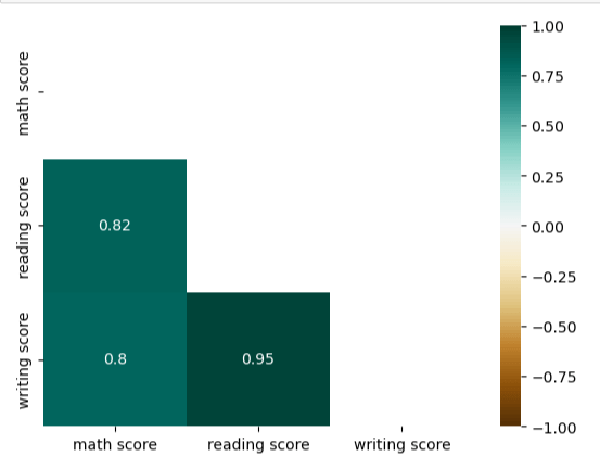
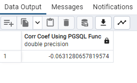
SELECT corr(“Area (km²)”, “Density (per km²)”) as “Corr Coef Using PGSQL Func”
FROM public.world_population;
ALTER TABLE public.world_population
ALTER COLUMN “Area (km²)” TYPE Numeric
USING “Area (km²)”::Numeric;
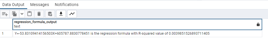
–the slope, intercept, and R-squared value of a linear regression model with “Area (km²)” as the independent variable and “Density (per km²)” as the dependent variable. The resulting regression formula and R-squared value would be returned as a string with the alias “regression_formula_output”.
The regr_slope() function is used to calculate the slope of the linear regression line, which represents the average change in the dependent variable (“Density (per km²)”) for a unit change in the independent variable (“Area (km²)”).
The regr_intercept() function is used to calculate the y-intercept of the linear regression line, which represents the value of the dependent variable when the independent variable is zero.
The regr_r2() function is used to calculate the R-squared value of the linear regression model, which represents the proportion of the variance in the dependent variable that is explained by the independent variable.
It is important to note that this query will only work if the database you are querying has a table called “world_population” with columns called “Area (km²)” and “Density (per km²)”. It is also important to make sure that the data in these columns are numeric and appropriate for calculating a linear regression model.–
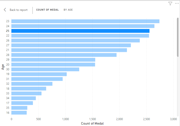
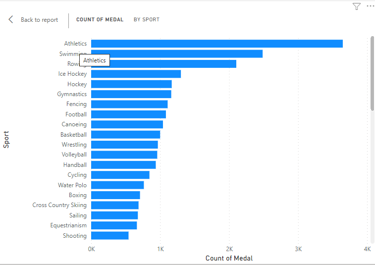
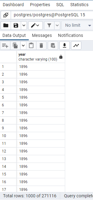
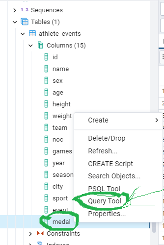
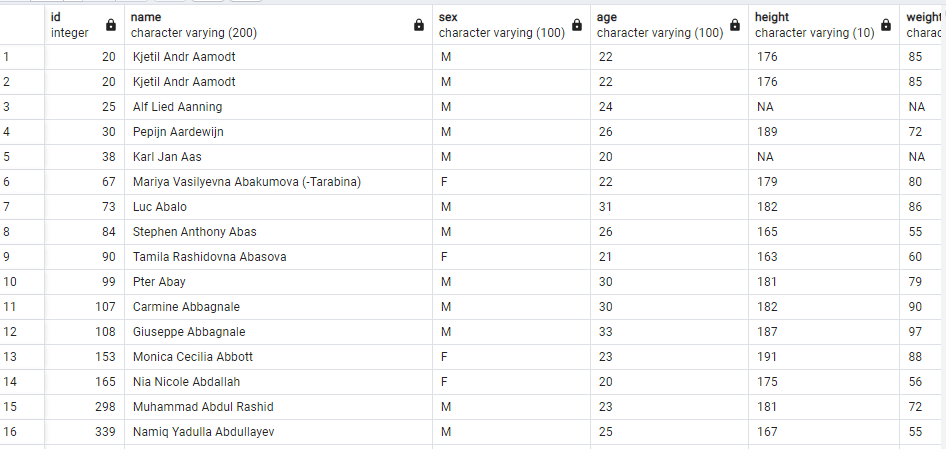
SportsStats (Olympics Dataset – 120 years of data)
A sports research company called SportsStats collaborates with professional personal trainers and local news outlets to offer “interesting” information that benefit their partners. For the aim of generating a news article or identifying important health insights, insights could be patterns or trends highlighting specific populations, occasions, or regions, among other things.
#Maximum count of medal has been earned by people in the age group of 23 years,
#Athletics and Swimming are the two sports for which maximum medals are awarded
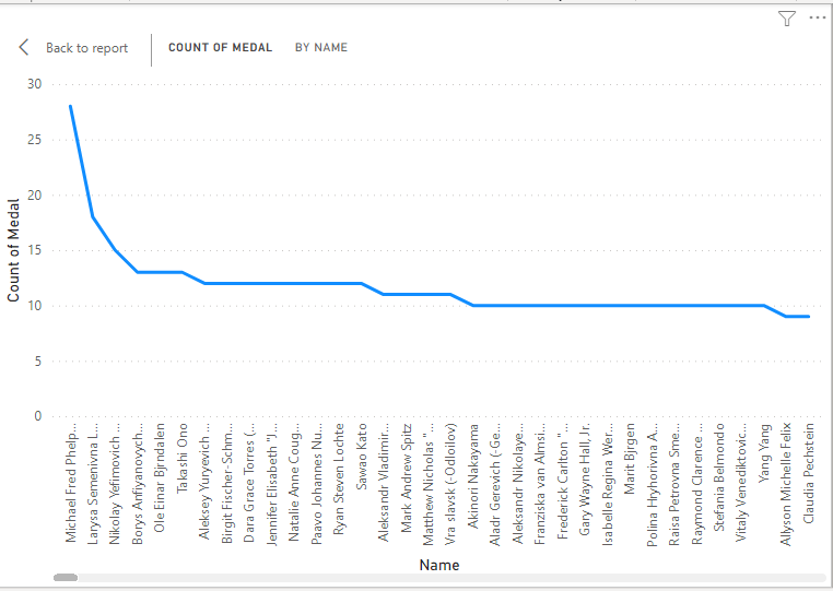
Michael Fred Phelp II has 28 Medals which is maximum!
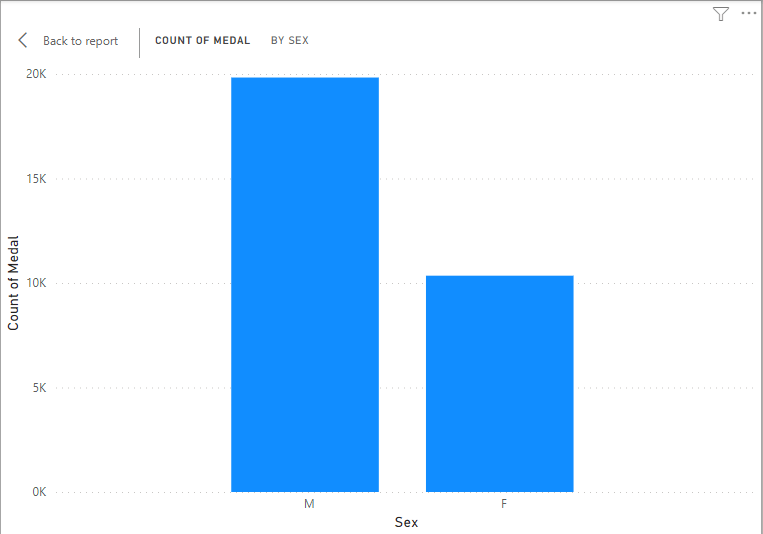
Male (19831Medals ) has more medals then females (10350 Medals)
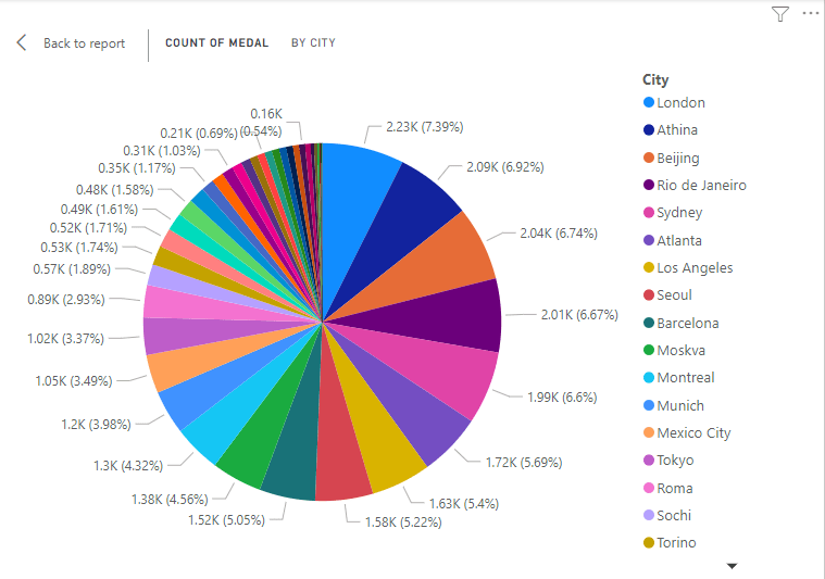
London city has the maximum number of medals ie. 2231 = 7.39%
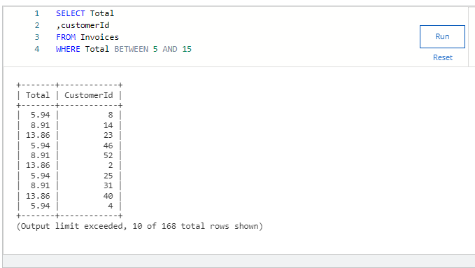
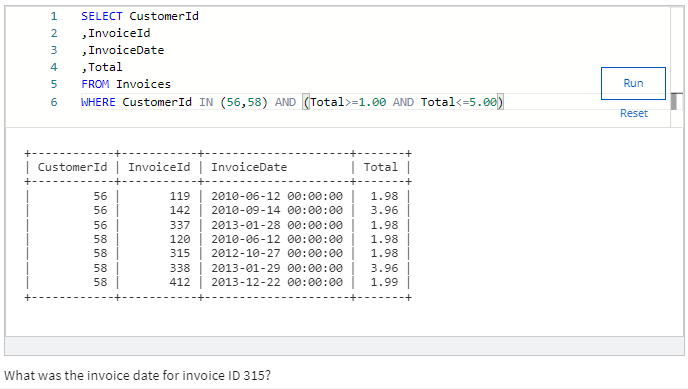
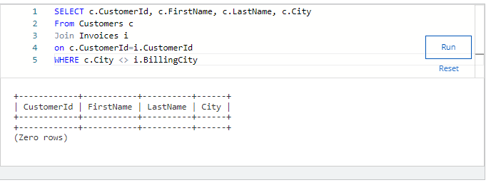
Run Query: Find all the invoices whose total is between $5 and $15 dollars.
While the query in this example is limited to 10 records, running the query correctly will indicate how many total records there are – enter that number below.
Answer = 168
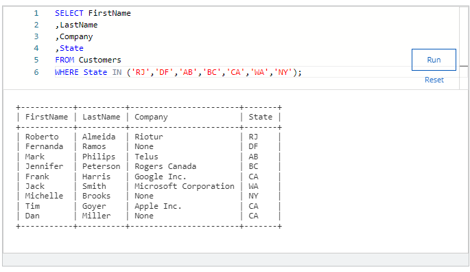
Run Query: Find all the customers from the following States: RJ, DF, AB, BC, CA, WA, NY.
What company does Jack Smith work for? 1 point
Microsoft Corp
Apple Inc.
Google Inc.
Rogers Canada
Answer : Microsoft Corp
My different code for the same question
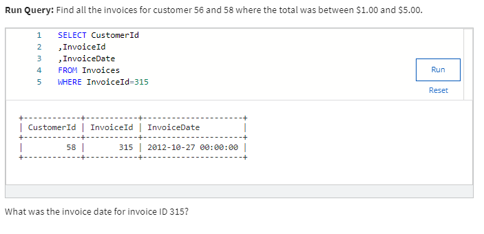
What was the invoice date for invoice ID 315?
Answer
10-27-2012
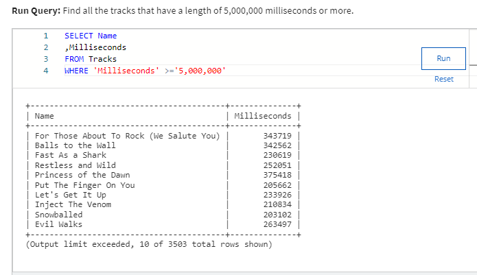
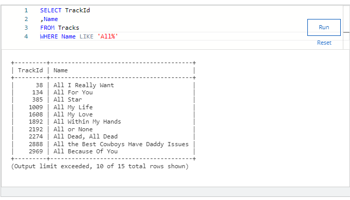
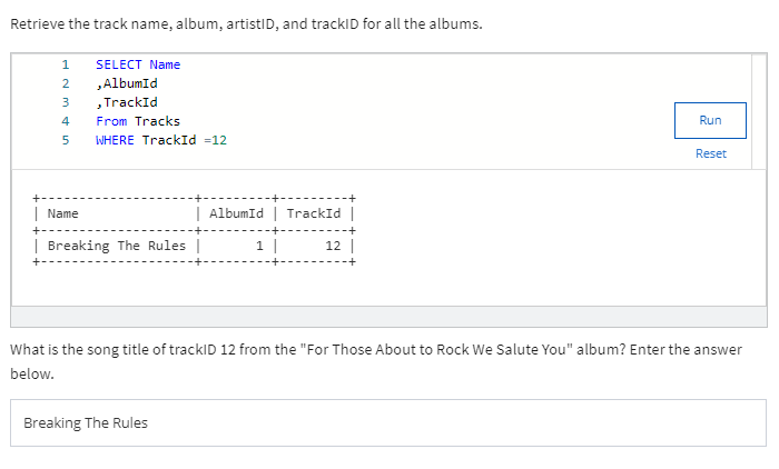
Run Query: Find all the tracks whose name starts with ‘All’.
While only 10 records are shown, the query will indicate how many total records there are for this query – enter that number below.
Answer = 15
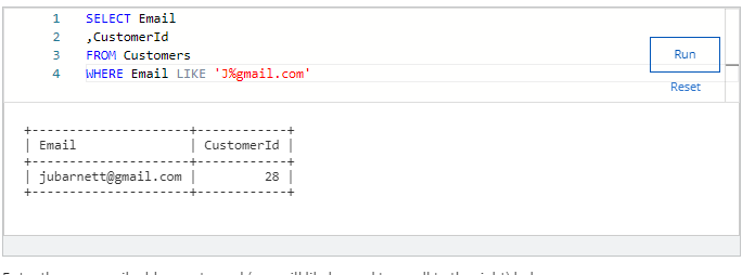
Run Query: Find all the customer emails that start with “J” and are from gmail.com.
Enter the one email address returned (you will likely need to scroll to the right) below.
Answer :
jubarnett@gmail.com
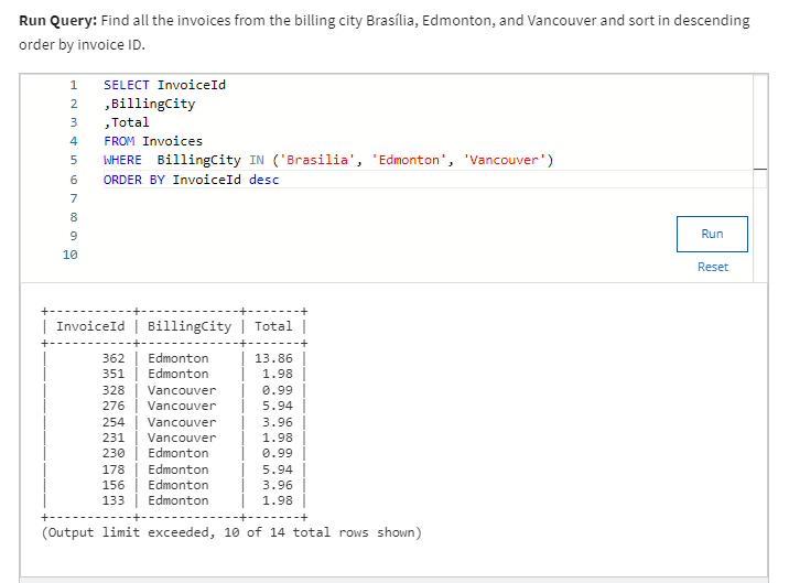
Run Query: Find all the invoices from the billing city Brasília, Edmonton, and Vancouver and sort in descending order by invoice ID.
What is the total invoice amount of the first record returned? Enter the number below without a $ sign. Remember to sort in descending order to get the correct answer.
Answer : 13.86
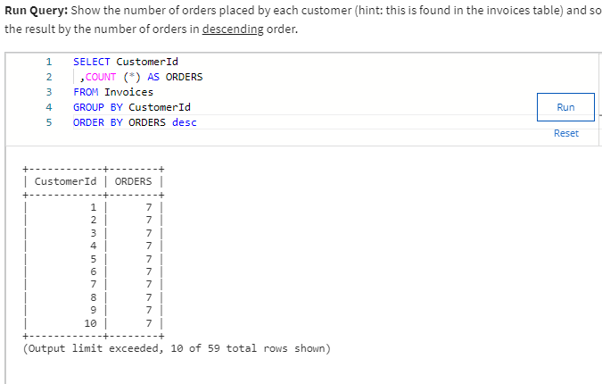
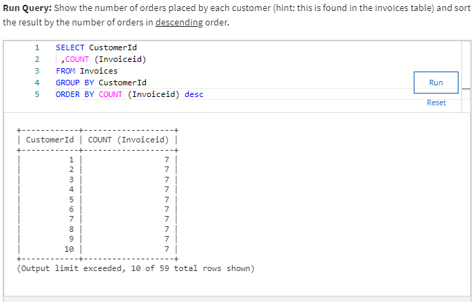
Run Query: Show the number of orders placed by each customer (hint: this is found in the invoices table) and sort the result by the number of orders in descending order.
What is the number of items placed for the 8th person on this list? Enter that number below.
Answer =7
Different code for the same question
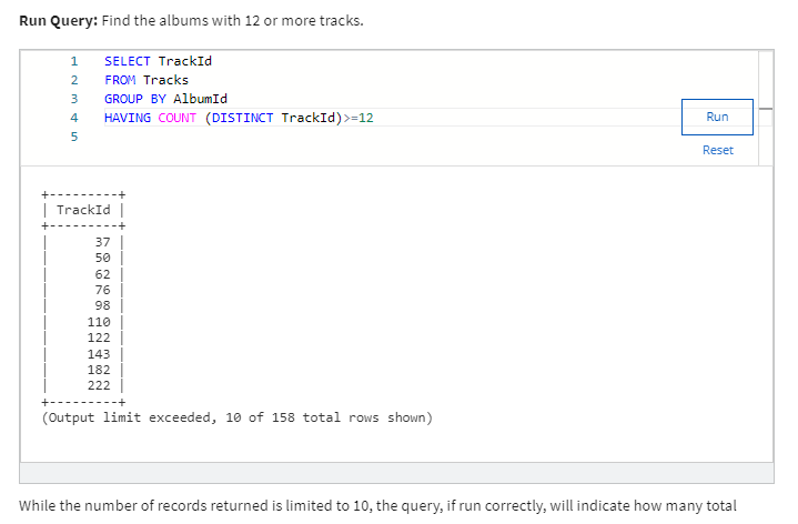
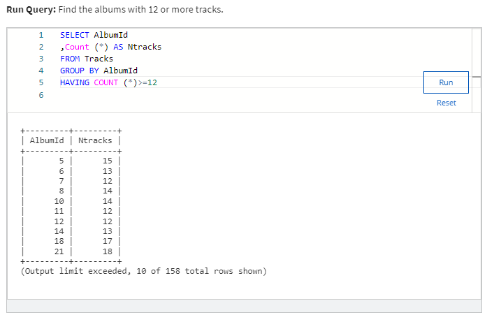
Run Query: Find the albums with 12 or more tracks.
While the number of records returned is limited to 10, the query, if run correctly, will indicate how many total records there are. Enter that number below.
Answer : 158
Same question by different code
MODULE 2 Questions
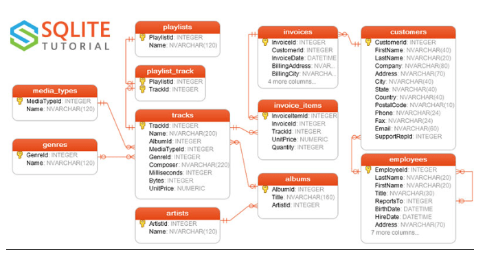
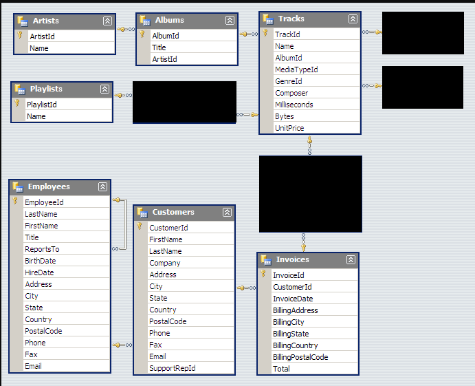
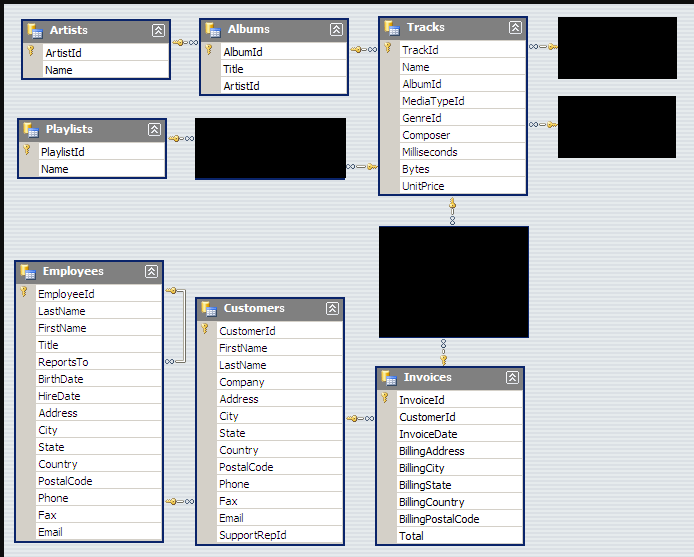
All of the questions in this quiz pull from the open source Chinook Database. Please refer to the ER Diagram below and familiarize yourself with the table and column names to write accurate queries and get the appropriate answers.
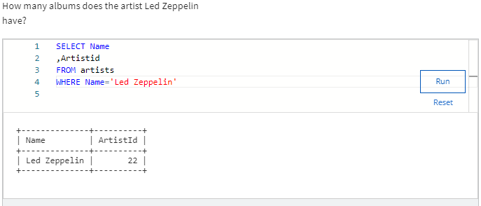
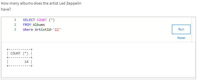
How many albums does the artist Led Zeppelin have?
Now Artist Led Zeppelin ID is 22
Here I used two codes to get the answer
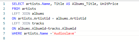
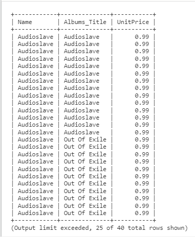
Create a list of album titles and the unit prices for the artist “Audioslave”.
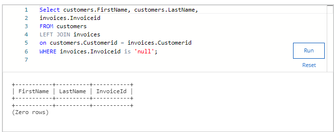
Find the first and last name of any customer who does not have an invoice. Are there any customers returned from the query?
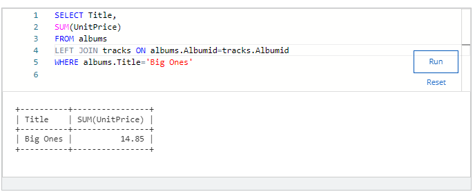
Find the total price for each album.
What is the total price for the album “Big Ones”?
ANS 14.85
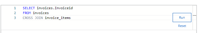
How many records are created when you apply a Cartesian join to the invoice and invoice items table?
Answer 922880
Module 3 Coding Assignment
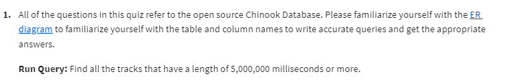
All of the questions in this quiz refer to the open source Chinook Database. Please familiarize yourself with the ER diagram in order to familiarize yourself with the table and column names in order to write accurate queries and get the appropriate answers.
Using a subquery, find the names of all the tracks for the album “Californication”.
ANS
8th track is
Porcelain
All of the questions in this quiz refer to the open source Chinook Database. Please familiarize yourself with the ER diagram in order to familiarize yourself with the table and column names in order to write accurate queries and get the appropriate answers.
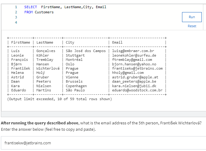
Find the total number of invoices for each customer along with the customer’s full name, city and email.
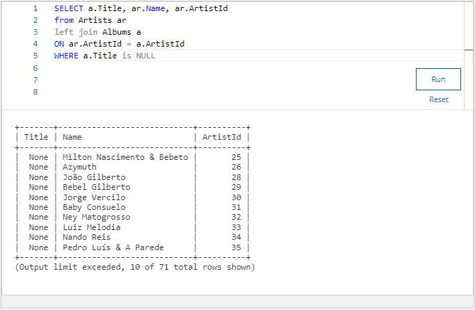
Find the name and ID of the artists who do not have albums.After running the query described above, two of the records returned have the same last name. Enter that name below.
Gilberto
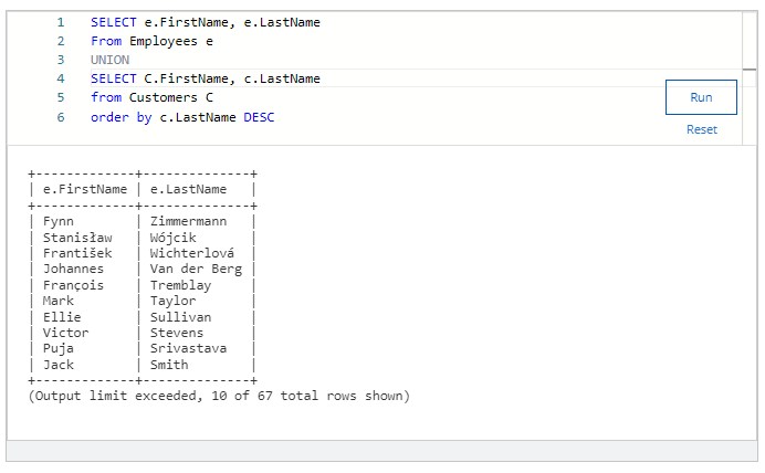
Use a UNION to create a list of all the employee’s and customer’s first names and last names ordered by the last name in descending order.
After running the query described above, determine what is the last name of the 6th record? Enter it below. Remember to order things in descending order to be sure to get the correct answer.
Taylor
See if there are any customers who have a different city listed in their billing city versus their customer city.
Answer
No customers have a different city listed in their billing city versus customer city.
Week 4 Quiz
All of the questions in this quiz refer to the open source Chinook Database. Please familiarize yourself with the ER diagram in order to familiarize yourself with the table and column names in order to write accurate queries and get the appropriate answers.
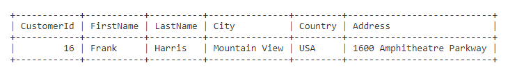
Pull a list of customer ids with the customer’s full name, and address, along with combining their city and country together. Be sure to make a space in between these two and make it UPPER CASE. (e.g. LOS ANGELES USA)
2.
Question 2
All of the questions in this quiz refer to the open source Chinook Database. Please familiarize yourself with the ER diagram in order to familiarize yourself with the table and column names in order to write accurate queries and get the appropriate answers.
Create a new employee user id by combining the first 4 letters of the employee’s first name with the first 2 letters of the employee’s last name. Make the new field lower case and pull each individual step to show your work.
SELECT FirstName,
LastName,
‘SUBSTR’ (FirstName, 1,4) AS A
‘SUBSTR'(LastName,1,2) AS B
‘SUBSTR'(FirstName,1,4)||’SUBSTR'(LastName,1,2) AS UserId
FROM Employees
What is the final result for Robert King?
RobeKi
All of the questions in this quiz refer to the open source Chinook Database. Please familiarize yourself with the ER diagram in order to familiarize yourself with the table and column names in order to write accurate queries and get the appropriate answers.
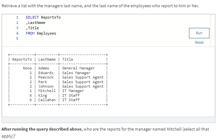
Show a list of employees who have worked for the company for 15 or more years using the current date function. Sort by lastname ascending.
What is the lastname of the last person on the list returned?
Peacock
All of the questions in this quiz refer to the open source Chinook Database. Please familiarize yourself with the ER diagram in order to familiarize yourself with the table and column names in order to write accurate queries and get the appropriate answers.
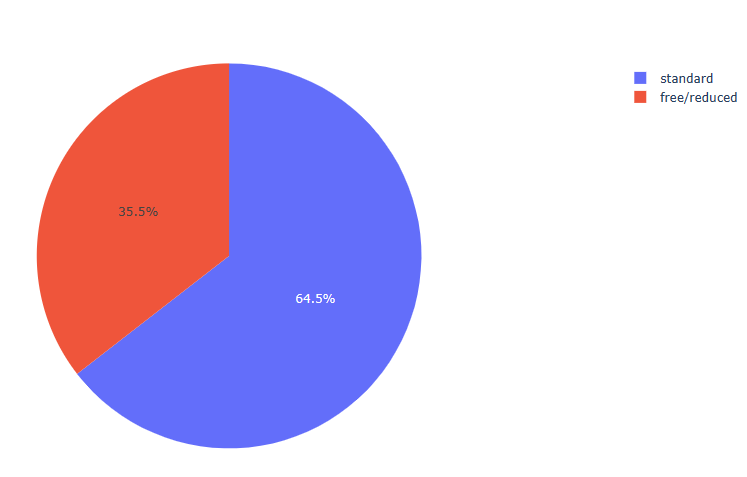
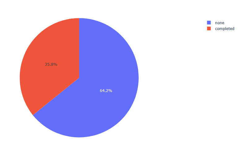
Profiling the Customers table, answer the following question.
SELECT COUNT(*)
FROM Customers
WHERE Phone IS NULL
FAX, Company, Phone , Postal code
All of the questions in this quiz refer to the open source Chinook Database. Please familiarize yourself with the ER diagram in order to familiarize yourself with the table and column names in order to write accurate queries and get the appropriate answers.
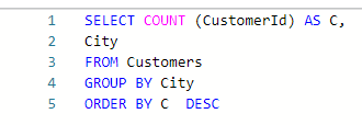
Find the cities with the most customers and rank in descending order.
ANS
London, Sao Paulo, Moutain View
All of the questions in this quiz refer to the open source Chinook Database. Please familiarize yourself with the ER diagram in order to familiarize yourself with the table and column names in order to write accurate queries and get the appropriate answers.
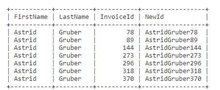
Create a new customer invoice id by combining a customer’s invoice id with their first and last name while ordering your query in the following order: firstname, lastname, and invoiceID.
Ans
Select all of the correct “AstridGruber” entries that are returned in your results below. Select all that apply.
SELECT Speed, CASE WHEN Speed > 50 THEN “below normal” WHEN Speed > 75 THEN “normal” WHEN Speed > 100 THEN “above normal” ELSE “below speed” END as “Speed_zone” FROM pokemon;
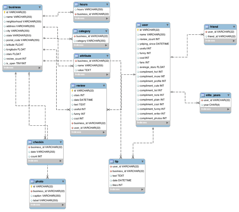
The entity-relationship (ER) diagram below, should help familiarize you with the design of the Yelp Dataset provided for this peer review activity.
Data Scientist Role Play: Profiling and Analyzing the Yelp Dataset Coursera Worksheet
This is a 2-part assignment. In the first part, you are asked a series of questions that will help you profile and understand the data just like a data scientist would. For this first part of the assignment, you will be assessed both on the correctness of your findings, as well as the code you used to arrive at your answer. You will be graded on how easy your code is to read, so remember to use proper formatting and comments where necessary.
In the second part of the assignment, you are asked to come up with your own inferences and analysis of the data for a particular research question you want to answer. You will be required to prepare the dataset for the analysis you choose to do. As with the first part, you will be graded, in part, on how easy your code is to read, so use proper formatting and comments to illustrate and communicate your intent as required.
For both parts of this assignment, use this “worksheet.” It provides all the questions you are being asked, and your job will be to transfer your answers and SQL coding where indicated into this worksheet so that your peers can review your work. You should be able to use any Text Editor (Windows Notepad, Apple TextEdit, Notepad ++, Sublime Text, etc.) to copy and paste your answers. If you are going to use Word or some other page layout application, just be careful to make sure your answers and code are lined appropriately. In this case, you may want to save as a PDF to ensure your formatting remains intact for you reviewer.
/* Are there any columns with null values in the Users table? Indicate “yes,” or “no.” Answer: “no”
SQL code used to arrive at answer:*/
SELECT id ,name ,review_count ,cool ,yelping_since ,useful ,funny ,fans ,average_stars FROM user WHERE id IS NULL OR name IS NULL OR review_count IS NULL ;
/*Please explain your findings and interpretation of the results:
Yes, but number three Harald does appear to be a significant anomaly. More “helpful” “cool” and “funny” reviews get more fans for the other users, but also in conjunction with the review count and length of time they have been yelping
Part 2: Inferences and Analysis
Pick one city and category of your choice and group the businesses in that city or category by their overall star rating. Compare the businesses with 2-3 stars to the businesses with 4-5 stars and answer the following questions. Include your code.
i. Do the two groups you chose to analyze have a different distribution of hours?
The 4-5 star group seems to have shorter hours then the 2-3 star group. Please note the query returned only three businesses so not a great sample size.
ii. Do the two groups you chose to analyze have a different number of reviews?
Yes and no, one of the 4-5 star group has a lot more reviews but then the other 4-5 star group has close to the same number of reviews as the 2-3 star group
iii. Are you able to infer anything from the location data provided between these two groups? Explain.
No, every business is in a different zip-code.
SQL code used for analysis:
SELECT business_id ,category FROM category GROUP BY category ORDER BY category=’%shopping%’;
Group business based on the ones that are open and the ones that are closed. What differences can you find between the ones that are still open and the ones that are closed? List at least two differences and the SQL code you used to arrive at your answer.
i. Difference 1:
The businesses that are open tend to have more reviews than ones that are closed on average.
Answer review count 35261 < 269300 so The businesses that are open tend to have more reviews
For this last part of your analysis, you are going to choose the type of analysis you want to conduct on the Yelp dataset and are going to prepare the data for analysis.
Ideas for analysis include: Parsing out keywords and business attributes for sentiment analysis, clustering businesses to find commonalities or anomalies between them, predicting the overall star rating for a business, predicting the number of fans a user will have, and so on. These are just a few examples to get you started, so feel free to be creative and come up with your own problem you want to solve. Provide answers, in-line, to all of the following:
i. Indicate the type of analysis you chose to do:
Predicting whether a business will stay open or close. We wish not to explicitly examine the text of the reviews, but this would be an interesting analysis.
ii. Write 1-2 brief paragraphs on the type of data you will need for your analysis and why you chose that data:
To better help businesses understand the importance of different factors which will help their business stay open. Some data that may be important; number of reviews, star rating of business, hours open, and of course location location location. We will gather the latitude and longitude as well as city, state, postal_code, and address to make processing easier later on. Categories and attributes will be used to better distinguish between different types of businesses. is_open will determine which business is open and which business have closed (not hours) but permanently.
iii. Output of your finished dataset:
SELECT id ,is_open ,stars ,review_count FROM business GROUP BY review_count ORDER BY review_count DESC LIMIT 20 ;
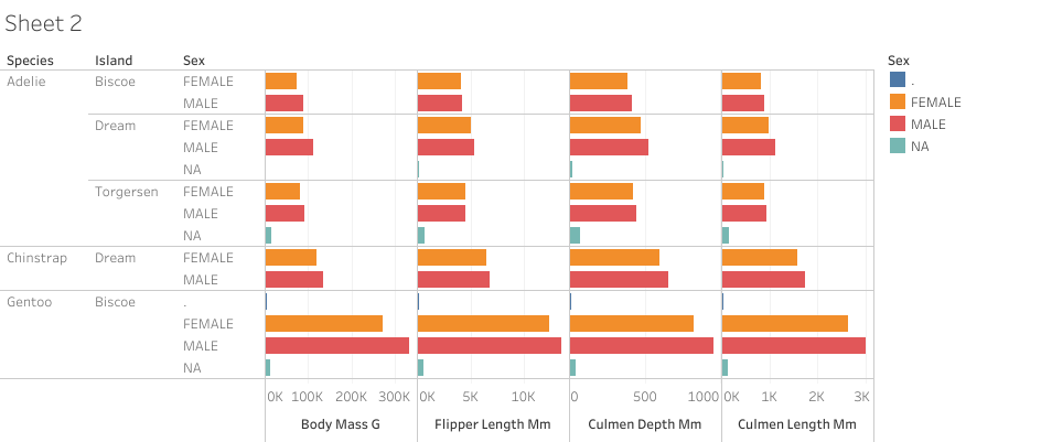
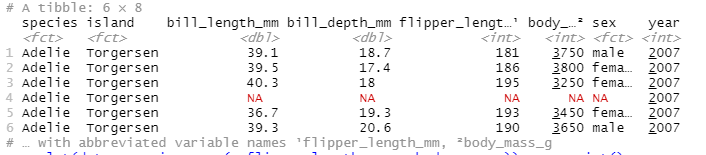
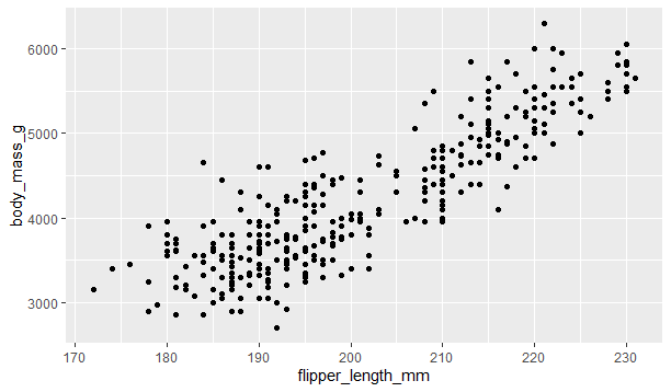
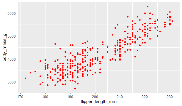
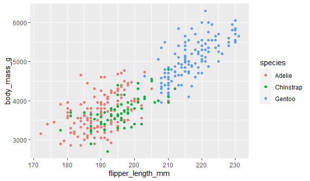
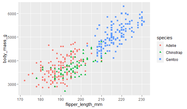
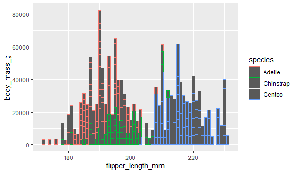
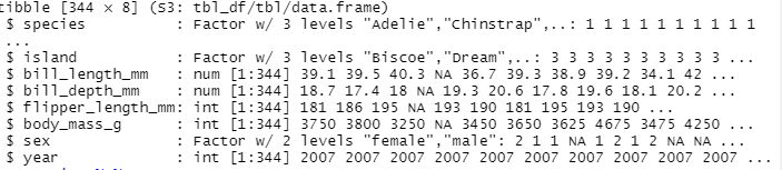
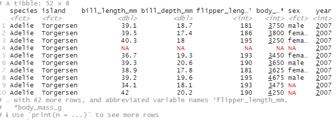
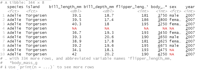
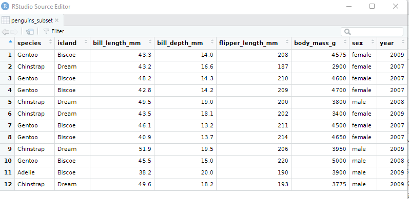
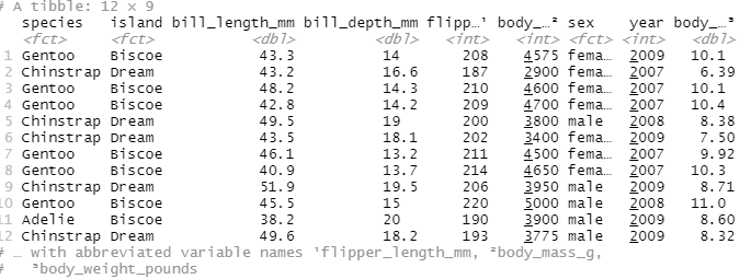
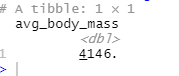
This week’s dataset involved deep diving into penguin habits to understand their body mass and other aspects:
The Palmer Penguins is a dataset constructed by Dr. Kirsten Gorman and relates to the structural size measurements of 3 species of penguins: adult, male and female Adelie, Chinstrap and Gentoo penguins. The data was collected at Palmer station Antarctica LTER between the period 2007-09. For each species, 4 structural size measurements were collected: bill length, bill depth, flipper length, and body mass. In total 344 samples were collected (however 2 samples have missing structural size measurements).
The data on the 3 different species of Penguins was collected from 3 islands in the Palmer archipelago in Antarctica. These islands are the Dream island, Torgerson island and Biscoe island
Of all the Palmer penguins, Gentoos are the largest. The second is Chinstrap and the last is Adelie.
Adelie species of Torgersen Island penguin’s male and female have negligible differentiation in body mass, flipper length, culmen depth, and culmen length
This mansion in the sought-after Villa Verde neighborhood will leave you speechless. With almost 3,000 square feet of area, you won’t be short on options. Enjoy movie night in your own personal media room, complete with sound wall panels for a cinematic experience. Work from home in the spacious study adjacent to the dining room at the front of the house. The living area has HIGH ceilings and LARGE windows. Relax on the rear patio, which is shaded and has a ceiling fan. A great area for grilling or a cup of coffee in the morning. Finally, unwind in the main bedroom and en suite, which includes a walk-in master closet. This property includes a tandem garage for EXTRA storage. *Buyers should do their homework and double-check dimensions.